9.3.2.   Mixtures by the RIfS Array

First, a multivariate calibration was performed using the sensor responses of all time points of all 4 sensors resulting in 200 independent variables. For the unsmoothed data, prediction errors of the validation data between 22.18% and 23.96% were achieved (see row 1 of table 7). The prediction errors of the validation data for the smoothed sensor signals are between 14.61% and 34.85% (see row 2 of table 7). When using the sensor signals of all 4 sensors no clear decision can be made if smoothing is beneficial for the calibration. As the 200 input variables contain too much redundant information for an optimal calibration, the parallel growing network framework (50 networks per analyte) was applied to the calibration data of the smoothed and the raw sensor signals. 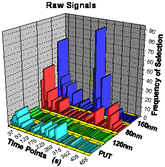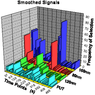The importance of the different variables is shown in figure 70 as frequency of selection. For the raw signals the 2 Makrolon sensors of 160 nm and 80 nm dominate, whereas the PUT sensor and the 120 nm Makrolon are by far less important. The variable ranking of the smoothed signals looks similar with two differences: Although the 160 nm and 80 nm sensors still dominate, the importance of the other two sensors increased and the important time points of the 80 nm sensor shifted from the end to the beginning of desorption. Compared with the 160 nm layer, the 80 nm layer has gained importance after smoothing.

figure 70:  Frequency of selection of the different variables after the first step of the parallel growing network framework.

The second step of the growing network framework stopped after the addition of 7 variables for the raw sensor signals and after the addition of 10 variables for the smoothed data. The variable selections for both data sets are similar and very astonishing. For both data sets, only time points of the 80 nm and of the 160 nm Makrolon layer are used. Additionally, only time points within the first 90 seconds of sorption and within the first 75 seconds of desorption are used (instead of 240 seconds of sorption and 210 seconds of desorption) suggesting that faster measurements are possible (see also discussion in section 10.3). Both, the predictions of the validation data and the predictions of the calibration data are significantly better for the raw and the smoothed data when compared with the calibrations using all time points of all sensors (see row 3 and row 4 of table 7). The quantification of methanol is better for the raw data, whereas the quantification of ethanol and 1-propanol is better for the smoothed data whereby for this combination of a thick and a thin layer no method can be generally preferred. 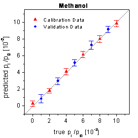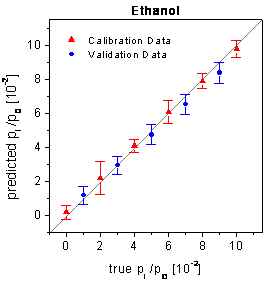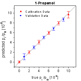The true-predicted plots for the raw data are shown in figure 71.

figure 71:  True-predicted plots for the raw sensor signals of the array setup whereby only the sensor responses of 2 sensors are evaluated.

In order to see the interactions of the thickness of layers and of smoothing, the sensor responses of the single sensors are calibrated using unoptimized networks (50 input neurons, 5 hidden neurons and 1 output neuron). The predictions of these single sensor calibrations for the raw and for the smoothed data are listed in row 5 to row 12 of table 7. First of all, the single sensor calibrations confirm the variable selection of the framework. The 160 nm layer shows the best calibrations whereas the PUT sensor and the 120 nm Makrolon sensor show poor calibrations. From the chemical point of view, the poor single sensor performance of the PUT sensor can be ascribed to the immediate sensor response without any time-resolution possible whereas the poor performance of the 120 nm Makrolon sensor cannot be explained.

The effect of smoothing is quite interesting for the 3 Makrolon layers with a different thickness. The 80 nm layer clearly benefits from the smoothing while the 160 nm layer shows worse calibration results if the smoothed sensor signals are used instead of the raw sensor signals. The 120 nm layer with the medium thickness shows no clear preference. The benefits of smoothing for thin layers can be explained by the improvement of the signal to noise ratio overcompensating the changes of the shapes of the sensor responses. On the other hand, the thick layers with a rather good signal to noise ratio are mainly affected by the disadvantageous changes of the shapes of the sensor signals without any real improvement of the signal to noise ratio.

table 7:      Relative RMSE for different data analysis methods and for different setups.